Part-3 Programming models in Warehouse-Scale Computing

sample image

Figure1 Spark & Python from http://static1.squarespace.com/static/538cea80e4b00f1fad490c1b/t/54b6b348e4b0a14bf3ec8b98/1421259603601/fast_data_apps.jpg

PREFACE

The goals of the articles today are to get you hands-on experience running MapReduce and gain a deeper understanding of the MapReduce paradigm, become more familiar with Apache Spark and get hands on experience with running Spark on a local installation and also learn how to apply the MapReduce paradigm to Spark by implementing certain problems/algorithms in Spark.

3.1 Quick Background

Apache Hadoop is an Open-source MapReduce Framework and also implements its own Hadoop Distributed File System (HDFS), both inspired by Google papers on their MapReduce and Google File System. For programming interface, Hadoop supports MapReduce Java APIs but it also has a big ecosystems (see Figure3 ), in which many other companies develop extensions, tools and higher-level programming platform to extend Apache Hadoop,

For example, you can also use other scripting languages like Python, JavaScript, Ruby or Groovy to control by the syntax similar to that of SQL for RDBMS systems through Apache Pig [1] developed by Yahoo.

sample image

Figure2 Apache Hadoop from https://i2.wp.com/hadoop.nl/hadoopelephant_rgb.png

sample image

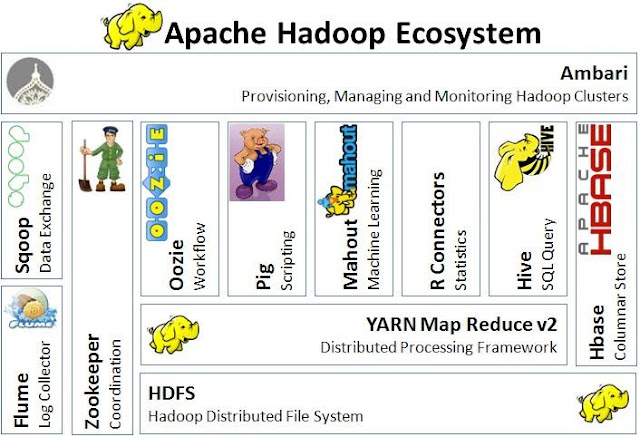
Figure3 Hadoop ecosystems from http://techblog.baghel.com/media/1/20130616-HadoopEcosystem.JPG

Despite the popularity of Hadoop, it has several disadvantages, for example, it doesn’t fit for small data and is vulnerable by nature due to its development language in Java. Therefore, when comes to big data, Hadoop may not the only answer. Apache Spark originally developed in the AMP lab at UC Berkeley is another choose offering fast and general engine for large-scale data processing, running on HDFS and providing Java, Scala, Python APIs for Database, Machine learning and Graph algorithm.

3.2 Setup Hadoop and Spark

Of course, environment setup sometime is really troublesome and time-consuming depending on your OS environments. So the fastest way to setup is to just use Amazon AWS EC2 but it’s also the most costly option. For practice purpose, installing them on local seems the most economical way you can do. However, notice both frameworks are in fact designed for running on cluster-level machines and processing a large-scale of data so you won’t expect the performance from distributing system and they could run much slower than local software to process the dataset when you install them as standalone mode.

As the focus today is to practice with the actual codes, to save the pages, I only leave the links below for setup depending on your local OS.

Hadoop on Mac, Linux and Windows: http://wiki.apache.org/hadoop/Running_Hadoop_On_OS_X_10.564-bit(Single-Node_Cluster) https://wiki.apache.org/hadoop/Hadoop2OnWindows
Spark setup on Mac, Linux and Windows: You can refer to the thread in StackOver http://stackoverflow.com/questions/25481325/how-to-set-up-spark-on-windows https://shellzero.wordpress.com/2015/07/24/how-to-install-apache-spark-on-mac-os-x-yosemite/
Spark and Hadoop in Amazon EC2 https://wiki.apache.org/hadoop/AmazonEC2 http://spark.apache.org/docs/latest/ec2-scripts.html

3.3 Run Spark on the command line

Actually running Spark with python file (xxx.py) is similar to how you run your Python files with python xxx.py), you just run the following command:

$ spark-submit xxx.py # Runs the Spark file xxx.py

If your Spark file takes in arguments (much like the Spark files we have provided), the command will be similar, but you will instead add however any arguments that you need, like:

$ spark-submit xxx.py arg1 arg2 # Runs the Spark file xxx.py and passes in arg1 and arg2 to xxx.py

Spark also includes this neat interpreter that runs with Python 2.7.3 and will let you test out any of your Spark commands right in the interpreter! The command is as follows:

$ pyspark # Runs the Spark interpreter.

If you want to preload some files (say a.py, b.py, c.py), you can run the following command:

$ pyspark --py-files a.py, b.py, c.py # Runs the Spark interpreter and you can now import stuff from a, b, and c

3.4 Practices

Ex1 – Generating the dataset

The fundamental idea we want to use WSC’s power through MapReduce framework is that we may have a huge workload that could be consumed couple days, months or even years to finish by using only one machine. Therefore, before starting to code the own map and reduce function, we need dataset.

In the examples, we’ll be working heavily with textual data and have some pre-generated datasets but it’s always more fun to use a dataset that you find interesting.

So this section, I’ll teach you guys how to generate the dataset from Project Gutenberg (a database of public-domain literary works) step by step.

I’ve put the code used in the following examples and data into my GitHub, Feel free to download from WSC_MapReduce-Spark

Head over to Project Gutenberg, pick a work of your choosing, and download the “Plain Text UTF-8” version into your lab directory. In this case, I pick EBook of Little Dorrit, by Charles Dickens in Figure4

sample image

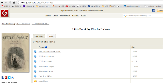
Figure4 EBook of Little Dorrit

Open up the file you downloaded in your favorite text editor and insert “—END.OF.DOCUMENT—” (without the quotes) by itself on a new line wherever you want Hadoop to split the input file into separate (key, value) pairs. The importer we’re using will assign an arbitrary key (like “doc_xyz”) and the value will be the contents of our input file between two “—END.OF.DOCUMENT—” markers.

sample image

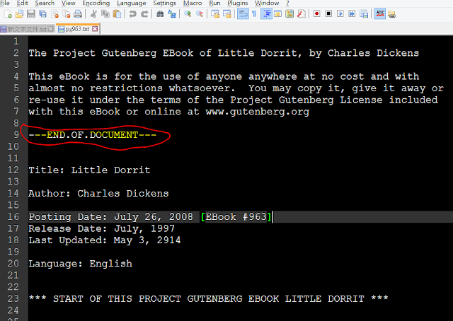
Figure5 insert “—END.OF.DOCUMENT—” in EBook

The importer is actually a MapReduce program which is used to convert TXT files into a Hadoop sequence file (the .seq extension). These are NOT human-readable. You can take a look at Importer.java if you want, but the implementation details aren’t important for this section.
We need to build out our importer JAR first by the following command in the console (in my folder, I’ve got these files, WordCount.java, pg963.txt, DocWordCount.java Importer.java and a folder /data/ and notice the paths of hadoop-core.jar and commons-cli.jar depend on your local installation.

javac -g -deprecation –cp /paul/hadoop/hadoop-core.jar:/paul/hadoop/lib/commons-cli.jar *.java jar cf wc.jar -C classe .

Now you can generate your input file like so:

hadoop jar wc.jar Importer YOUR_FILE_FROM_STEP_2.txt

Your generated .seq file can now be found in the convertedOut directory

sample image

Figure6 convertedOut directory

Ex2 – Running Word Count

Here we use the common-seen example word. Open WordCount.java you will see the codes adapted from the http://wiki.apache.org/hadoop/WordCountHadoopwiki

What here basically do is to define mapper class – WordCountMap and reducer class – SumReduce, and then create a job object to represent a wordcount Job and tell Hadoop where to locate the code that must be shipped if this job is to be run across a cluster. And then set all the required tasks and parameters before we start, such as datatypes of the keys and values outputted by the maps and reduces and set the mapper, combiner, reducer to use. You can see the comments in the following code snippet for more info.

Code snippet of WordCount.java:

public static class WordCountMap extends Mapper {
        /** Regex pattern to find words (alphanumeric + _). */
        final static Pattern WORD_PATTERN = Pattern.compile("\\w+");

        /** Constant 1 as a LongWritable value. */
        private final static LongWritable ONE = new LongWritable(1L);

        /** Text object to store a word to write to output. */
        private Text word = new Text();

        @Override
        public void map(Text key, Text value, Context context)
                throws IOException, InterruptedException {
            Matcher matcher = WORD_PATTERN.matcher(value.toString());
            while (matcher.find()) {
                word.set(matcher.group());
                context.write(word, ONE);
            }
        }
    }

  public static class SumReduce extends Reducer {
        @Override
        public void reduce(Text key, Iterable values,
                Context context) throws IOException, InterruptedException {
            long sum = 0L;
            for (LongWritable value : values) {
                sum += value.get();
            }
            context.write(key, new LongWritable(sum));
        }
    }


public static void main(String[] rawArgs) throws Exception {
        /* Use Hadoop's GenericOptionsParser, so our MapReduce program can accept
         * common Hadoop options.
         */
        GenericOptionsParser parser = new GenericOptionsParser(rawArgs);
        Configuration conf = parser.getConfiguration();
        String[] args = parser.getRemainingArgs();

        /* Create an object to represent a Job. */
        Job job = new Job(conf, "wordcount");

        /* Tell Hadoop where to locate the code that must be shipped if this
         * job is to be run across a cluster. Unless the location of code
         * is specified in some other way (e.g. the -libjars command line
         * option), all non-Hadoop code required to run this job must be
         * contained in the JAR containing the specified class (WordCountMap
         * in this case).
         */
        job.setJarByClass(WordCountMap.class);

        /* Set the datatypes of the keys and values outputted by the maps and reduces.
         * These must agree with the types used by the Mapper and Reducer. Mismatches
         * will not be caught until runtime.
         */
        job.setMapOutputKeyClass(Text.class);
        job.setMapOutputValueClass(LongWritable.class);
        job.setOutputKeyClass(Text.class);
        job.setOutputValueClass(LongWritable.class);

        /* Set the mapper, combiner, reducer to use. These reference the classes defined above. */
        job.setMapperClass(WordCountMap.class);
        job.setReducerClass(SumReduce.class);

        /* Set the format to expect input in and write output in. The input files we have
         * provided are in Hadoop's "sequence file" format, which allows for keys and
         * values of arbitrary Hadoop-supported types and supports compression.
         *
         * The output format TextOutputFormat outputs each key-value pair as a line
         * "keyvalue".
         */
        job.setInputFormatClass(SequenceFileInputFormat.class);
        job.setOutputFormatClass(TextOutputFormat.class);

        /* Specify the input and output locations to use for this job. */
        FileInputFormat.addInputPath(job, new Path(args[0]));
        FileOutputFormat.setOutputPath(job, new Path(args[1]));

        /* Submit the job and wait for it to finish. The argument specifies whether
         * to print progress information to output. (true means to do so.)
         */
        job.waitForCompletion(true);
    }

Now, we can see the result by compile and package the .java source file into a .jar and then run it on our desired input (we use pre-built data as example - data/billOfRights.txt.seq but you can replace it with your seg file).

hadoop jar wc.jar WordCount data/billOfRights.txt.seq wc-out-wordcount-small

This will run WordCount over billOfRights.txt.seq. Your output should be visible in wc-out-wordcount-small/part-r-00000. If we had used multiple reduces, the output would be split across part-r-[id.num], where Reducer “id.num” outputs to the corresponding file. The key-value pair for your Map tasks is a document identifier and the actual document text.

sample image

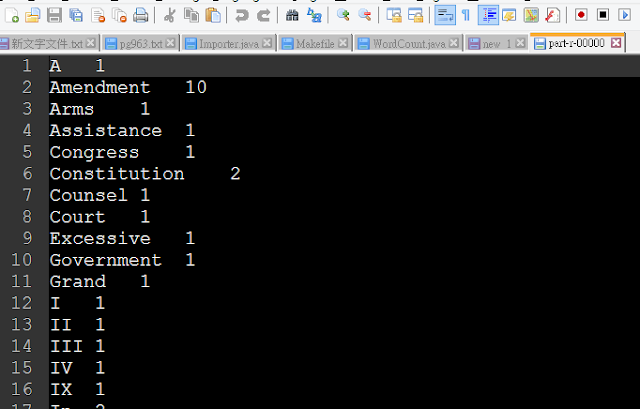
Figure7 the result of word count over billOfRights.txt.seq in part-r-00000.

For simplifying the compiling process, we create a Makefile. Instead, you can just run the following make command for the same result as above.

$ make wordcount-small

Next, try your code on the larger input file complete-works-mark-twain.txt.seq. In general, Hadoop requires that the output directory not exist when a MapReduce job is executed, however our Makefile takes care of this by removing our old output directory.

Ex3 – Document Word Count

Now is you turn to play around MapReduce. Open DocWordCount.java. Notice that it currently contains the same code as WordCount.java (but with modified class names), which you just compiled and tried for yourself. Modify it to count the number of documents containing each word rather than the number of times each word occurs in the input - for example, the word “Affery” appears in six documents rather than 66 times of occurrence in the all documents.

Academy 1 Affairs 2 Affery 6 After 10 Again 3

Code snippet of DocWordCount.java:

@Override
        public void map(Text key, Text value, Context context)
                throws IOException, InterruptedException {

            /* MODIFY THE BELOW CODE */

        }
    }

    public static class SumReduce extends Reducer {

        @Override
        public void reduce(Text key, Iterable values,
                Context context) throws IOException, InterruptedException {

  /* MODIFY THE BELOW CODE */

        }
    }

You can test DocWordCount using either of the following (for our two data sets):

$ make docwordcount-small # Output in wc-out-docwordcount-small/

$ make docwordcount-medium # Output in wc-out-wordcount-medium/

Ex4 –Working with Spark

Now that you have gained some familiarity with the MapReduce paradigm, we will shift gears into Spark and investigate how to do what we did in the previous exercise in Spark! I have provided a complete wordcount.py, to get you a bit more familiar with how Spark works. To help you with understanding the code, I have added some comments, but feel free to check out transformations and actions on the Spark website for a more detailed explanation on some of the methods that can be used in Spark.

def wordcount(file_name, output="spark-wc-out-wordcount"):
    sc = SparkContext("local[8]", "WordCount")
    """ Reads in a sequence file FILE_NAME to be manipulated """
    file = sc.sequenceFile(file_name)

    """
    - flatMap takes in a function that will take one input and outputs 0 or more
      items
    - map takes in a function that will take one input and outputs a single item
    - reduceByKey takes in a function, groups the dataset by keys and aggregates
      the values of each key
    """
    counts = file.flatMap(flat_map) \
                 .map(map) \
                 .reduceByKey(reduce)

    """ Takes the dataset stored in counts and writes everything out to OUTPUT """
    counts.coalesce(1).saveAsTextFile(output)

To get you started on implementing DocWordCount.java in Spark, we have provided a skeleton file docwordcount.py.

def flat_map(document):
    """
    Takes in document, which is a key, value pair, where document[0] is the
    document ID and document[1] is the contents of the document.
    """
    """ Your code here. """
    return re.findall(r"\w+", document[1])

def map(arg):
    """ Your code here. """
    return (arg, arg)

def reduce(arg1, arg2):
    """ Your code here. """
    return arg1

To test your docwordcount.py, you can run either of the following two commands:

$ make sparkdwc-small # Output in spark-wc-out-docwordcount-small/

$ make sparkdwc-medium # Output in spark-wc-out-docwordcount-medium/

Ex5 – Working with Spark

Open index.py. Notice that the code is similar to docwordcount.py. Modify it to output every word and a list of locations (document identifier followed by the word index of EACH time that word appears in that document). Make sure your word indices start at zero. Your output should have lines that look like the following:

(word1 document1-id, word# word# …) (word1 document2-id, word# word# …) . . . (word2 document1-id, word# word# …) (word2 document3-id, word# word# …) . . . Notice that there will be a line of output for EACH document in which that word appears and EACH word and document pair should only have ONE list of indices. Remember that you need to also keep track of the document ID as well.

For this exercise, you may not need all the functions we have provided. If a function is not used, feel free to remove the method that is trying to call it. Make sure your output for this is sorted as well (just like in the previous exercise.

def flat_map(document):
    """
    Takes in document, which is a key, value pair, where document[0] is the
    document ID and document[1] is the contents of the document.
    HINT: You need to keep track of three things, word, document ID, and the
    index inside of the document, but you are working with key, value pairs.
    Is there a way to combine these three things and make a key, value pair?
    """
    """ Your code here. """
    return re.findall(r"\w+", document[1])

def map(arg):
    """ Your code here. """
    return (arg, arg)

def reduce(arg1, arg2):
    """ Your code here. """
    return arg1

You can test index.py by using either of the following commands (for our two datasets):

$ make index-small # Output in spark-wc-out-index-small/

$ make index-medium # Output in spark-wc-out-index-medium/

The output from running make index-medium will be a large file. In order to more easily look at its contents, you can use the commands cat, head, more, and grep:

$ head -25 OUTPUTFILE # view the first 25 lines of output

$ cat OUTPUTFILE | more # scroll through output one screen at a time (use Space)

$ cat OUTPUTFILE | grep the # output only lines containing 'the' (case-sensitive)

3.3 Solution

I put all the solutions for the examples above in the folder named solutions here.

let me know if you have any other further questions.